Source code please see in Github repository
Q1 Fuzzy Clustering using EM
Given the training data EM Points.mat, you should implement the Fuzzy Clustering using EM algorithm for clustering.
The dataset contains 400 2D points totally with 2 clusters. Each point is in the format of [Xcoordinate, Y-coordinate, label].
You are required to implement Fuzzy Clustering using the EM algorithm.
- You are NOT allowed to use any existing EM library. You need to implement it manually and submit your code.
- Report the updated centers and SSE for the first two iterations. (If you set any hyper parameter when computing SSE, please write it clearly in the report.)
- Report the final converged centers for each cluster.
- In your report, draw the clustering results of your implemented algorithm and compare it with the original labels in the dataset. You need to discuss the result briefly.
Hint: For terminate condition, you can consider the change of parameters or the max iterations.
1 | import numpy as np |
1 | points = loadmat("EM_Points.mat")["Points"] |
array([[-0.3005007 ,  0.71622977,  0.        ],
       [-0.07260801,  1.39849283,  0.        ],
       [-0.209947  ,  1.32075583,  0.        ],
       ...,
       [ 1.42954638,  0.15714956,  1.        ],
       [ 1.14187298, -0.21691986,  1.        ],
       [ 1.49161487, -0.50410824,  1.        ]])
Assume $o_i$ represents the i-th object and $c_j$ represents the j-th center. The sum of the squared error is computed by
1 | class FuzzyClusteringEM: |
1 | initc = np.array([[1,1],[2,2]]) |
iteration = 0
SSE = 452.2064066190702
C =
[[0.53866521 0.55193537]
 [0.47385793 0.60978921]]

iteration = 1
SSE = 209.93907719136445
C =
[[0.60141888 0.46557221]
 [0.43167368 0.63543004]]

iteration = 2
SSE = 205.38336884149535
C =
[[0.7256404  0.32912566]
 [0.3051053  0.77335614]]

iteration = 3
SSE = 183.55466797593803
C =
[[0.90598324 0.1294149 ]
 [0.11855499 0.9793926 ]]

iteration = 4
SSE = 148.13131455149812
C =
[[1.01083941 0.01034638]
 [0.00611246 1.09897161]]

iteration = 5
SSE = 137.8432366754871
C =
[[ 1.03788056 -0.02172753]
 [-0.02550994  1.12770828]]

iteration = 6
SSE = 137.1701001910947
C =
[[ 1.04306219 -0.02775795]
 [-0.03212375  1.13224185]]

iteration = 7
SSE = 137.14633312924246
C =
[[ 1.0440722  -0.02874075]
 [-0.03347604  1.13280377]]

iteration = 8
SSE = 137.14555718757154
C =
[[ 1.04429125 -0.02887354]
 [-0.03377623  1.13283733]]

iteration = 9
SSE = 137.14552695547323
C =
[[ 1.04434439 -0.02888064]
 [-0.03385258  1.13282462]]

iteration = 10
SSE = 137.14552517019524
C =
[[ 1.04435838 -0.02887534]
 [-0.03387519  1.13281695]]

iteration = 11
SSE = 137.14552500427823
C =
[[ 1.04436222 -0.02887173]
 [-0.0338828   1.13281404]]

iteration = 12
SSE = 137.14552498415927
C =
[[ 1.04436327 -0.02886999]
 [-0.0338856   1.13281311]]

iteration = 13
SSE = 137.1455249813707
C =
[[ 1.04436355 -0.02886921]
 [-0.03388668  1.13281284]]

iteration = 14
SSE = 137.1455249809489
C =
[[ 1.04436361 -0.02886888]
 [-0.03388712  1.13281277]]
We set two initial centroids
In the first three iterations, the updated centers and SSE
| Iteration | Updated Centers | SSE |
|---|---|---|
| 0 | 452.206 | |
| 1 | 209.939 | |
| 2 | 205.383 |
After about 10 iterations, we can get the final converged centers
with $SSE = 137.145$
1 | pred_labels = clustering.labels_ |
1 | fig = plt.figure(figsize=(15,4)) |
According to the figures we draw, we can clearly see that predicted clustering has a more distinct boundary than the clutering divided by original labels. I have drawed the clutering boundary below:
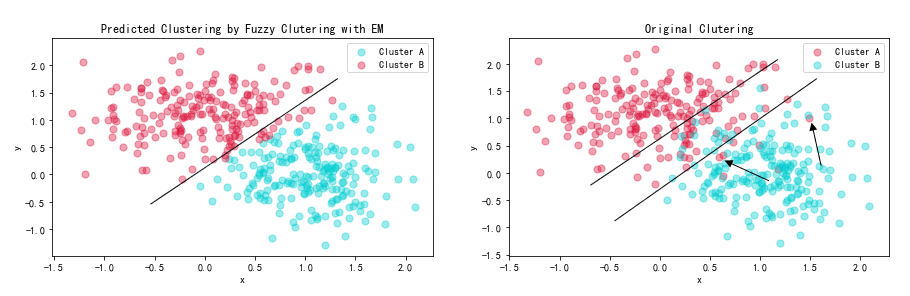
We can easily draw a line to distinguish two cluters in the left figure. However, in the figure on the right, though we widen the boundary, there are still some outliers existing. This is because in reality, the noise exists which would make some points fluctuate near the classification boundary. However, The algorithm just consider the ideal situation and cannot consider noise.
Q2 DBSCAN
Given the dataset DBSCAN.mat with 500 2D points, you should apply DBSCAN algorithm to
cluster the dataset and find outliers as the following settings:
Parameter Setting
- Set $\epsilon$ = 5, Minpoints=5.
- Set $\epsilon$ = 5, Minpoints=10
- Set $\epsilon$ = 10, Minpoints=5.
- Set $\epsilon$ = 10, Minpoints=10.
Implementation
- Draw a picture for your cluster results and outliers in each parameter setting in your report. For clearly, in each picture, the color of outliers should be BLUE.
- Add a table to report how many clusters and outliers you find in each parameter setting in your report.
- Discuss the results of different parameter settings, and report the best setting that you think and write your reason clearly.
- Note that you are NOT allowed to use any existing DBSCAN library. You need to submit your code.
1 | import random |
1 | points = loadmat("DBSCAN.mat")["Points"] |
1 | class DBSCAN: |
1 | eps_list = [5, 10] |
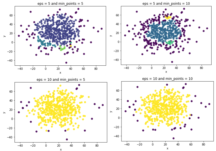
From the figures above, we could see that the outliers are mainly distributed in the edge area, which shown in dark BLUE. When using parameters eps = 10 and min_points = 5, the clusters are clear and distinct with less number of outliers. If the parameters are set as eps = 5 and min_points = 10, the number of outliers are up to 198. Not very well.
The detailed results are shown in the table:
| eps | min_points | n_clusters | n_outliers |
|---|---|---|---|
| 5 | 5 | 5 | 71 |
| 5 | 10 | 3 | 198 |
| 10 | 5 | 1 | 20 |
| 10 | 10 | 1 | 33 |