MSBD 6000G Deep Learning Meets Computer Vision, BDT, HKUST
Start on October 18, 2019: Project Proposal PDF
Finish on December 8, 2019: Project Final Report PDF
Group Members: YANG Rongfeng, YIN Dongxin
abstract
Computer vision has been introduced to extract information from the give images, such as food classification. However, current food image data set do not contain a volume and mass records of food, which leads to an incomplete calorie estimation. In this paper, we introduce a data set generated by Y. Liang and J. Li in 2017. There are 2978 images in this data set and every image contains corresponding each foods annotation, volume and mass records, as well as a certain calibration reference. To detect the food objects and segment objects from the background, we do some research in two deep learning methods to figure out: Faster R-CNN and Mask R-CNN. However, Faster R-CNN need to be combined with GrabCut algorithm to get each food’s contour. After getting the instance segmented, food’s volume and calorie can be calculated by the given mass and energy records. The experiment results made from two different methods are comparable and both prove that our estimation is effective.
1 Introduction
With the improvement of living standards, the obesity rate is also growing rapidly reflecting people’s health risks. People need to control their daily calorie intake by eating healthier, which is the most basic way to avoid obesity. However, obese patients often have trouble balancing their calorie intake and consumption due to lack of relevant nutritional information or other reasons. Despite the nutritional and calorie labels on the food packaging, it is still not very convenient for costumers to refer to. Therefore, developing a computer vision-based measurement method is beneficial to people who want to lose weight in a healthy way and keep a healthy lifestyle.
Convolution neural network has been widely used to image classification and object detection. Compared with image classification, the object detection is a more challenging task since the increase of model complexity. Complexity arises because detection requires the accurate localization of objects, creating two primary challenges. First, numerous candidate object locations must be processed. Second, these candidates provide only rough localization that must be refined to achieve precise localization. Solutions to these problems often compromise speed, accuracy, or simplicity.
Recently, many ideas have been proposed to detect food energy and the key to calorie estimation is the choice of calibration. W. Jia, H. C. Chen, et al use circle plate as their calibration of model. In another research, thumb is also used as calibration object by Gregorio Villalobos et al. However, these approaches are not popularized because its self-limitation and instability. More specifically, the plate is not portable in many cases and the human thumb could have different size. Therefore, we need to select a calibration with common and stable attributes.
1.1 R-CNN
The Region-based Convolutional Neural Network method (R-CNN) is one of the state-of-the-art CNN-based deep learning object detection approach and has achieved excellent object detection accuracy by using a deep CNN to classify object proposals. However, R-CNN has a bad performance in terms of time and space consuming. Firstly, it uses a CNN on object proposals. Then SVM models and bounding-box regression models are trained to fit CNN features. Whether in at training time or testing time, the features are extracted from each object proposal in each image. The process is slow and occupy to much storage.
1.2 Object Detection
Object detection means predict the concept and localization of the target to gain a complete image comprehension. The main tasks of object detection are to determine where the objects are located in the given images and which categories the objects belong to. The whole process can be divided into three parts: information region selection, feature extraction and classification.
Information region selection. Considering the fact that objects may locate on the different regions with various sizes, it is natural to take multi-scale sliding windows. Quite a few useless windows are created to cover all the possible locations which indicate expensive computation waste. However, if we reduce the scan scale by limit the window choice, the prediction accuracy cannot be promised. How to tradeoff between the computational cost and satisfactory prediction is still a challenge.
Feature extraction. To recognize different objects, we need to extract visual features by convolutional neural networks. A set of learnable filters are used to train a feature descriptor.
The representation is susceptible to the image content, such as occlusion, illumination conditions and background clutter etc. A good feature extraction model must be invariant to the cross product of all these variations, while simultaneously retaining sensitivity to the inter-class variations.
Classification. After selecting information regions and extracting features, it is worth classifying the object from a set of categories to recognize a visual concept. There are various classifiers such as Nearest Neighbor Classifier, Linear Classifier and Support Vector Machine (SVM). In Linear Classifier, each classifier has two major components: a score function that maps the raw data to class scores, and a loss function that quantifies the agreement between the predicted scores and the ground truth labels. It is optimized by minimizing the loss function with respect to the parameters of the score function.
1.3 Semantic Segmentation
Semantic segmentation refers to the process of classifying each pixel of the images of what is being represented. The process of semantic segmentation follows an encoder and decoder structure where we down-sample the spatial resolution of input to develop lower-resolution feature mappings and up-sample the feature representations to gain a full-resolution segmentation map. So far some exiting and well-studied image classification networks without fully connected layers have been introduced to encode the input image into feature maps. It has been proven that adding skip connections to sum the feature maps can provide necessary details to reconstruct accurate shapes for segmentation boundaries. Semantic segmentation is very useful in various areas, including GPS, autonomous vehicles and medical image diagnostics.
2 Dataset
Though Food-101, PFID and FOODD can be introduced to train and test object detection algorithms, it is still hard to utilize them to estimate calories just because they have not prepared the volume and mass as a reference. The ECUSTFD dataset which is provided by J. Li. and Y. Liang is designed to estimate calories.
2.1 Dataset Description
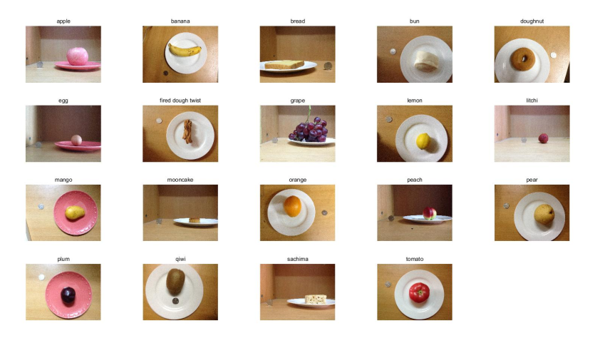
ECUSTFD is a free public food image dataset. This dataset contains 19 kinds of food: apple, banana, bread, bun, doughnut, egg, fired dough nut, grape, lemon, litchi, mango, mooncake, orange, peach, pear, plum, qiwi, sachima and tomato. Some example images are shown in the figure. The total number of images is 2978. Each food target has a top view and a side view. There is only a One Yuan coin as calibration object and no more than two food in each image. In spite of the image data, the dataset also provides mass, density and energy records which are used to calculate calories with predicted volume.
2.2 Shooting Conditions
Relative factors that affect the accuracy of estimation results: viewpoint, illumination, background and food type.
Viewpoint. Each food contains pictures of two angles: top view and side view. When taking a top view, shooting angle is almost 0 degree from the table; and when taking a side view, shooting angle is almost 90 degree from the table.
Illumination. Considering lighting influence the detection significantly, the images in the dataset are taken from different illumination conditions. For instance, some photos are taken in the dark environment with or without flash.
Background. As objects may appear with backgrounds in a diversity, it is a natural choice to take pictures with various backgrounds. In most cases, food is put on a red or white plate; in other cases, food is placed on the dining table directly.
Food type. Foods are selected with large volume and not liable to deform. Since estimating targets with small volumes is really hard and will be easy to cause great error compared with the measured ground truth.
3 Faster R-CNN
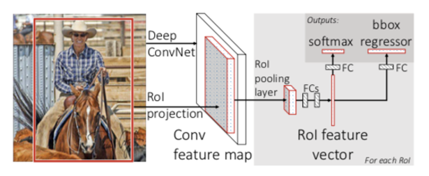
In the following figure, faster R-CNN architecture takes an image and multiple object proposals as input. The image will be put into a convolution neural network with convolutional layers and max pooling layers to extract a feature map. Then, for each object proposal, a region of interest (RoI) pooling layer produce a fixed-length feature vector from the feature map. Each feature vector is fed into a sequence of fully connected layers that finally branch into two sibling output layers: one that produces softmax probability estimating over K object classes and another layer that outputs four real-valued numbers for each of the K object classes. Each set of 4 values encodes refined bounding-box positions for one of the K classes.
3.1 The RoI Pooling Layer
The RoI pooling layer uses max pooling to convert the features inside any valid region of proposal into a small feature map with a fixed spatial extent of $H \times W$ where H and W are hyper-parameters that are independent of any particular RoI. Each RoI is defined by a four-tuple $(r, c, h, w)$ that specifies its top-left corner $(r, c)$ and its height and width $(h, w)$. RoI max pooling works by dividing the $h \times w$ RoI window into an $H \times W$ grid of sub-windows of approximate size $\frac{h}{H} \times \frac{w}{W}$ and then max pooling the values in each sub-window into the corresponding output grid cell.
3.2 Initializing with pre-trained networks
Faster R-CNN is constructed on the pre-trained ImageNet networks, each with five max pooling layers and between five and thirteen convolutional layers. When a pre-trained network initializes a Fast R-CNN network, it undergoes three transformations.
First, Fast R-CNN not only an image but also a set of proposals as input.
Second, the last max pooling layers is replaced by RoI pooling layer with a pair of hyper-parameter H and W to define a fixed window size.
Third, the network’s last fully connected layer and softmax are modified to two sibling output layers: softmax for classification and regression for bounding-box positions.
3.3 Mini-batch sampling and SGD
Back-propagation through R-NN network is highly inefficient when each training sample comes from a different image. The inefficiency stems from the fact that each RoI may have a very large receptive field, often spanning the entire input image.
In Faster R-CNN, back-propagation is more efficient by taking advantage of stochastic gradient descent (SGD) with mini-batches during training, first by sampling N images and then by sampling $\frac{R}{N}$ RoIs from each image. Critically, RoIs from the same image share computation and memory in the forward and backward passes. Making N small decreases mini-batch computation.
3.4 Scale invariance
Faster R-CNN achieve scale invariant object detection in two ways: “brute force” learning and by using image pyramids.
In the brute-force approach, each image is processed at a pre-defined pixel size during both training and testing. The network must directly learn scale-invariant object detection from the training data.
The multi-scale approach, in contrast, provides approximate scale-invariance to the network through an image pyramid. At test-time, the image pyramid is used to approximately scale-normalize each object proposal. During multi-scale training, Faster R-CNN randomly sample a pyramid scale each time an image is sampled as a form of data augmentation.
4 GrabCut
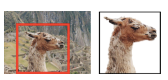
The figure shows how GrabCut works. GrabCut provides a powerful and iterative way to segment the foreground and background in each image with bounding-box annotations.
4.1 Color data modeling
The image is taken to consist of pixels in RGB color space. As it is impractical to construct adequate color space histograms, GrabCut follows a practice that is already used for soft segmentation and use GMMs. Each GMM, one for the background and one for the foreground, is taken to be a full-covariance Gaussian mixture with K components. In order to deal with the GMM tractably, in the optimization framework, an additional vector $k={k_1,…,k_n,…,k_N}$ is introduced, with $k_n \in {1,…,K}$, assigning, to each pixel, a unique GMM component, one component either from the background or the foreground model, according as $\alpha_n = 0$ or 11.
4.2 Segmentation by iterative energy minimization
The new energy minimization scheme in GrabCut works iteratively, in place of the previous one-shot algorithm. This has the advantage of allowing automatic refinement of the opacities, as newly labelled pixels from the region of the initial trimap are used to refine the color GMM parameters $\theta$.
The first step of GrabCut system is straightforward, done by simple enumeration of the $k_n$ values for each pixel $n$. Step 2 is implemented as a set of Gaussian parameter estimation procedures, as follows. For a given GMM component $k$ in, say, the foreground model, the subset of pixels is defined. The mean and covariance are estimated in standard fashion as the sample mean and covariance of pixel values. Finally step 3 is a global optimization, using minimum cut.
The structure of the algorithm guarantees proper convergence properties. This is because each of steps 1 to 3 of iterative minimization can be shown to be a minimization of the total energy E. E decreases monotonically, so the algorithm is guaranteed to converge at least to a local minimum of E. It is straightforward to detect when E ceases to decrease significantly, and to terminate iteration automatically.
4.3 User interaction and incomplete trimaps
The iterative minimization algorithm allows increased versatility of user interaction. In particular, incomplete labelling becomes feasible where, in place of the full trimap $T$, the user needs only specify, say, the background region $T_B$, leaving the foreground region $T_F=0$. No hard foreground labelling is done at all. Iterative minimization deals with this incompleteness by allowing provisional labels on some pixels which can subsequently be retracted; only the background labels $T_B$ are taken to be firm guaranteed not to be retracted later and the initial $T_B$ is determined by the user as a strip of pixels around the outside of the marked rectangle.
The initial, incomplete user-labelling is often sufficient to allow the entire segmentation to be completed automatically, but by no means always. If not, further user editing is needed, it takes the form of brushing pixels, constraining them either to be firm foreground or firm background; then the minimization step 3. is applied. Note that it is sufficient to brush, roughly, just part of a wrongly labeled area. In addition, the optional “refine” operation updates the color models, following user edits. This propagates the effect of edit operations which is frequently beneficial. Note that for efficiency the optimal flow, computed by Graph Cut, can be re-used during user edits.
5 Calories Estimation Process}
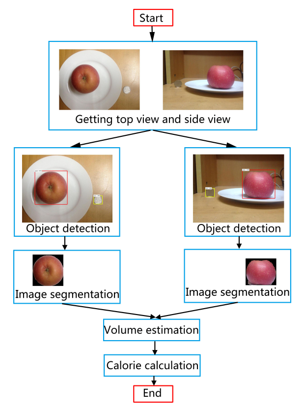
The process of calories estimation has three step as the figure shown. First, we need to detect the object by Faster R-CNN. Then segmented object pixels are got after applying GrabCut to the bounding boxes from Faster R-CNN. At last, we would estimate the volume of each object and then calculate their calories.
5.1 Object Detection by Faster R-CNN
As we described before, Faster R-CNN network takes an image and a set of proposals as input and output a sequence of bounding boxes with specific classification.
After detecting objects from the top view, we can get a sequence of bounding boxes $box_T^1,box_T^2,\dots,box_T^n$. For $i^{th}$ ($i \in 1, 2,\dots, n$) bounding box $box_T^i$, the food category is $type_T^i$. Besides, we regard the bounding box $c_T$ with the highest score as the calibration object to compute the top view scale factor.
In a similar way, we detect the objects from the side view to get a sequence of bounding boxes $box_S^1,box_S^2,\dots,box_S^m$. For $j^{th}$ ($j \in 1, 2,\dots, m$) bounding box $box_S^j$, the food category is $type_S^j$. Finally, the bounding box $c_S$ with the highest score as the calibration object is used to compute the top view scale factor.
5.2 Image Segmentation with GrabCut
After detecting the objects, we apply GrabCut algorithm to handle each bounding box generated from Faster R-CNN networks. GrabCut segment the object in the bounding box from the background by replacing the values of the background pixels with zero. The image $P_T^i (i \in 1, 2,\dots, n)$ which is the output of GrabCut algorithm has the same size with $box_T^i$, indicating that GrabCut only remains the object pixels values while set the background values to zero.
5.3 Volume Estimation
To estimate volume of each object, we need to calculation the scale factor depending on the detected calibration. When we use the One Yuan coin as the reference, according to the coin’s real diameter(2.50 cm), we can calculate the side view’s scale factor $\alpha_S$ (cm) with Equation 1.
\noindent where $W_S$ is the width of the bounding box $c_S$ and $H_S$ is the height of the bounding box $c_S$.
Then, the top view’s scale factor $\alpha_T$ (cm) is calculated by Equation 2.
\noindent where $W_T$ is the width of the bounding box $c_T$ and $H_T$ is the height of the bounding box $c_T$.
For each food image $P_T^i (i \in 1, 2,\dots, n)$, we aim to find an image in set $P_S^1,P_S^2,\dots,P_S^m$ with the same food category. If $type_T^i$ equals to $type_S^j (j \in 1, 2,\dots, m)$, $P_S^j$ will be marked to calculate this food’s volume with $P_T^j$. We divide objects into three shape types: ellipsoid, column, irregular. According to the food type $type_T^i$, we select the corresponding volume estimation formula as shown in Equation 3.
In Equation 3, $H_S$ is the number of rows in side view $P_S$ and $L_S^k$ is the number of foreground pixels in row $k (k \in 1, 2, \dots, H_S)$. $L_S^{MAX} = max(L_S^1,L_S^2,\dots,L_S^{H_S})$ records the maximum number of foreground pixels in $P_S \cdot S_T=\sum_{k=1}^{H_T}L_T^k$ is the number of foreground pixels in top view $P_T$, where $L_T^k$ is the number of foreground pixels in row $k (k \in 1, 2, \dots, H_T)$. $\beta$ is the compensation factor and the default value is 1.
5.4 Calorie Estimation
After getting volume of the object, we get down to estimate the corresponding mass with Equation 4.
where $v(cm^3)$ is the volume of current food and $\rho (g/cm^3)$ is the density value.
Finally, each food’s calorie is calculated by Equation 5.
where $m(g)$ is the mass of current food and $c(Kcal/g)$ is its calories per gram.
6 Experiment
Our experiment is done in the environment:
- Matlab + matcaffe + VS2013 + cuda65 + cudnn + opencv2.49
- Faster R-CNN project
Our project is tested on Windows 10 x64 with Navida Geforce 940MX.
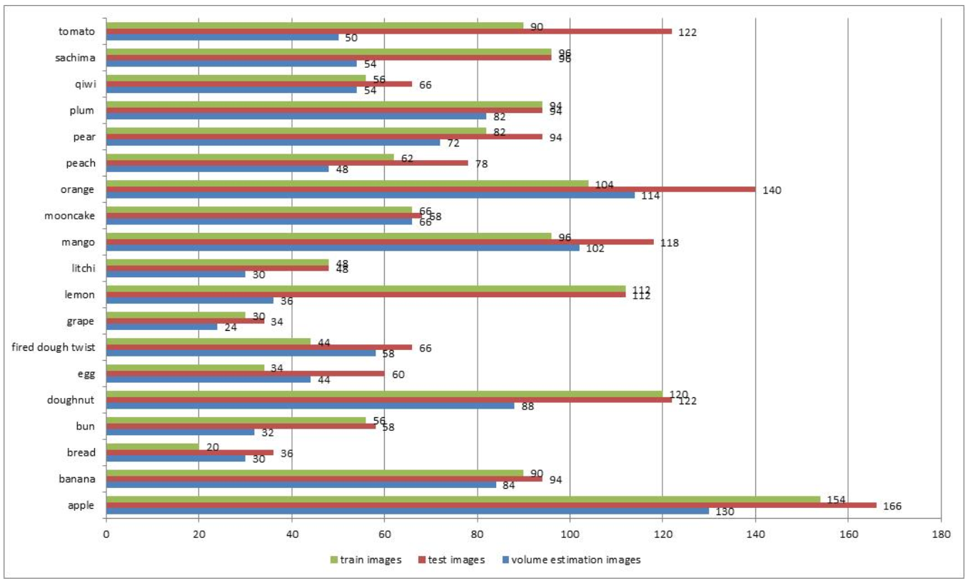
In this section, we present the volume estimation results using the food images dataset. These food and fruit images are divided into train and test sets. In order to avoid using train images to estimate volumes, the images of two sets are not selected randomly but orderly. The numbers of train and test images used for Faster R-CNN are listed in Figure 5. After Faster R-CNN is well trained, we use those pairs of test images which Faster R-CNN correctly recognizes to estimate volumes. In other words, those images Faster R-CNN cannot identity or misidentify in test sets will be discarded. The numbers of images in volume estimation experiments are shown in Figure~\ref{fig:Image Number in Experiment} either. The code can be downloaded at this website. We use mean error to evaluate volume estimation results. Mean error ME is defined as:
In Equation 6, for food type $i$ , $n_i$ is the number of images Faster R-CNN recognizes correctly. Since we use two images to calculate volume, so the number of estimation volumes for $i^{th}$ type is $n_i$. $v_j$ is the estimation volume for the $j^{th}$ pair of images with the food type $i$; and $V_j$ is corresponding estimation volume for the same pair of images.
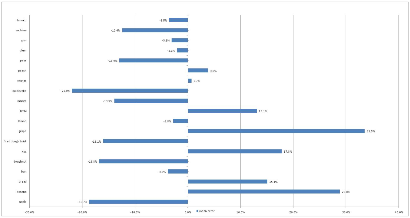
Volume estimation results are shown in Figure~\ref{fig:Volume Estimation Results}. For most types of food in our experiment, the estimation volume are closer to reference volume. The mean error between estimation volume and true volume does not exceed $\pm 20\%$ except banana, grape, mooncake. For some food types such as orange, our estimation result is close enough to the true value. As for the bad estimation results of grape, the way we measure volumes of grapes should be to blame. When measuring grapes’ volumes, we have not used plastic wrap to cover grapes but put them into the water directly, so the volumes we estimated are far from the reference values because of the gaps. All in all, our estimation method is available.
7 Conclusion
In this paper, we provided our calorie estimation method. Our method needs a top view and side view as its inputs. Faster R-CNN is used to detect the food and calibration object. GrabCut algorithm is used to get each food’s contour. Then the volume is estimated with volume estimation formulas. Finally we estimate each food’s calorie. The experiment results show our method is effective.