6000G course is Deep Learning Meets Computer Vision that I learnt in HKUST Fall semester in the first year. The course focuses on image process in Machine Learning. Its teaching materials are from Standford cs231n course Convolutional Neural Networks for Visual Recognition including its PPT, lecture notes, example codes and assignments.
After doing each assignment, I’ll mark down my thoughts, questions, solutions and other interesting things here.
The all assignments are divided into three parts:
- Assignment #1: Image Classification, kNN, SVM, Softmax, Neural Network
- Assignment #2: Fully-Connected Nets, Batch Normalization, Dropout, Convolutional Nets
- Assignment #3: Image Captioning with Vanilla RNNs, Image Captioning with LSTMs, Network Visualization, Style Transfer, Generative Adversarial Networks
Prepare
The course has pre-prepared the virtual barn ( Adv. GPU Pool ) for our each student via the VMWare Horizon Client and VPN. However using this win10 system to do the experiment, I found that it works even worse than my own laptop, slower speed and delayed reponse. Thus I went back to my local environment.
The full package of assignment materials run on win10 and contain the python 3.6, jupyter notebook, WinPy, IDLE and etc. You just easily click your mouse to open jupyter, and then begin to work without scratching your head to configure the environment.
The assignment can be described as code complement : With the algorithm skeleton codes given, you need to complete them. You always require numpy to help you express matrix, to calculate some parameters like loss, gradient, accuracy, relative error, to tune hyper-parameter or to compare different model. Some inline questions are asked to make you think the reason behind a phenomenon. No matter what the problem is, you have to understand the backgound knowledge of each ML model. Otherwise you don’t know how to start.
Assignment One
At the first step I downloaded the experiment data ( CIFAR-10 image data set with labels ) by running getdata.py. Then I noticed the main structure with tutorial is in .ipynb file which calls functions from some .py files. The first difficulty I met was numpy broadcast features in knn no-loop algorithm. It’s also comfused me that the direction of axis = 0 or axis = 1 and the effect of keepdims = True.
The other obstacles I encountered are as follows :
- How to calculate the loss function?
- How to calculate the gradient of loss function?
- How to tune the hyper-parameter in neural network?
- The principle of features extraction?
- The different way to process the image between raw pixels and features ( HOG + color histogram ).
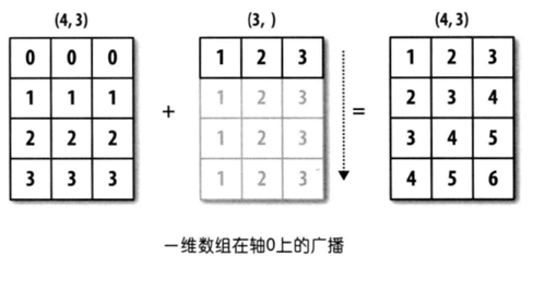
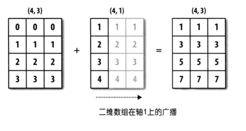
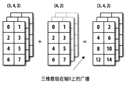
1.1 numpy boardcast
These three pictures show a clear view how numpy broadcast works.
1.2 axis and keepdims
1 | x = np.array([[0, 2, 1], |
The output1
2
3
4
5
6
7
812
[1 5 6]
[3 9]
[[3]
[9]]
1.3 How to calculate loss and the gradient of it?
SVM
We have a training set X ( n samples with d dimensions ) to train a model i.e. learning a W ( d dimensions and c classes ) . The y contains the real label of each sample in X. S is the scores matrix to evaluate the quality of our model i.e. finding the ideal W.
We see that $s_{ij}$ shows that the $i^{th}$ sample score performing in the $j^{th}$ class. And we calculate the loss using following expression:
Notice that we may get zero sometimes, we consider that the $i^{th}$ row of $(S - S[:,y].broadcast + 1)$ maxtrx has $k_i$ none-zero values. And this $k_i$ values columns numbers are $t_{1}^i,t_{2}^i,\dots,t_{k_i}^i$. So the loss expression can rewrite to
We can calculate the derivative of loss with respect to W and get a $d\times c$ matrix ( gradient matrix ). Initialize
Then let
If we want to add regularization, we can let
and the gradient need to add
Softmax
The way to calculate Matrix S is same to SVM. However Softmax uses softmax value to calculate the loss and gradient. We use P maxtrix to express the softmax formula. This is
Then we make
In order to avoid numeric instability when we do exp and log, we would minus the max score in each row like this
Then we get $P’$ like $S$ to $P$. The loss
To simple the illustration, we use $S$ and $P$ to express $S’$ and $P’$. Notice that we make $S = S’,P = P’$.
It’s easy to think that
Do partial derivative
Let’s take one part to see more details,
if $j=y[1]$ then
if $j\neq y[1]$ then
Consider the two different situation $j=y[1]$ and $j\neq y[1]$. Make
Then we’ll find that ( here we do partial derivative to $W$; we do partial derivative to $w_{ij}$ ahead )
So the gradient