Machine Learning HW1 Solution

文章目录

1. 1. Question 1
2. 2. Question 2
3. 3. Question 3
4. 4. Question 4
   1. 4.1. use raw features
   2. 4.2. add an additional feature
5. 5. Question 5

ML-HW1 PDF
Update on October 4, 2019: ML-HW1 Solution PDF

Question 1

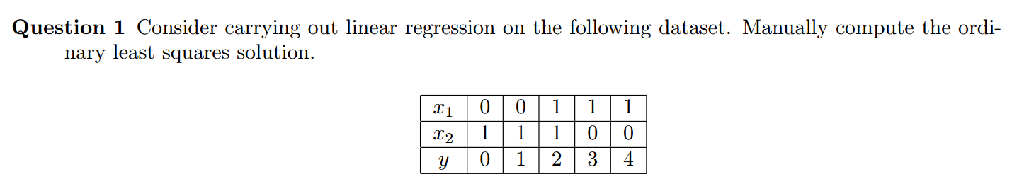
According to the known condition, make $x_0=1$ i.e. add a column with 1 in matrix $X$:

$$X = \begin{bmatrix} 1 & 0 & 1\\ 1 & 0 & 1\\ 1 & 1 & 1\\ 1 & 1 & 0\\ 1 & 1 & 0 \end{bmatrix} \quad y = \begin{bmatrix} 0 \\ 1 \\ 2 \\ 3 \\ 4 \end{bmatrix}$$

The OLS solution:

$$\begin{aligned} \hat{W} &= (X^TX)^{-1} \cdot X^T \cdot y \\ &= \left(\begin{bmatrix} 1 & 1 & 1 & 1 & 1\\ 0 & 0 & 1 & 1 & 1\\ 1 & 1 & 1 & 0 & 0\\ \end{bmatrix} \cdot \begin{bmatrix} 1 & 0 & 1\\ 1 & 0 & 1\\ 1 & 1 & 1\\ 1 & 1 & 0\\ 1 & 1 & 0 \end{bmatrix}\right)^{-1} \cdot \begin{bmatrix} 1 & 1 & 1 & 1 & 1\\ 0 & 0 & 1 & 1 & 1\\ 1 & 1 & 1 & 0 & 0 \end{bmatrix} \cdot \begin{bmatrix} 0 \\ 1 \\ 2 \\ 3 \\ 4 \end{bmatrix}\\ &= \begin{bmatrix} 5 & 3 & 3\\ 3 & 3 & 1\\ 3 & 1 & 3 \end{bmatrix}^{-1} \cdot \begin{bmatrix} 1 & 1 & 1 & 1 & 1\\ 0 & 0 & 1 & 1 & 1\\ 1 & 1 & 1 & 0 & 0 \end{bmatrix} \cdot \begin{bmatrix} 0 \\ 1 \\ 2 \\ 3 \\ 4 \end{bmatrix}\\ \end{aligned}$$ $$\begin{aligned} \hat{W} &= \begin{bmatrix} 2 & -3/2 & -3/2\\ -3/2 & 3/2 & 1\\ -3/2 & 1 & 3/2 \end{bmatrix} \cdot \begin{bmatrix} 1 & 1 & 1 & 1 & 1\\ 0 & 0 & 1 & 1 & 1\\ 1 & 1 & 1 & 0 & 0 \end{bmatrix} \cdot \begin{bmatrix} 0 \\ 1 \\ 2 \\ 3 \\ 4 \end{bmatrix}\\ &= \begin{bmatrix} 1/2 & 1/2 & -1 & 1/2 & 1/2\\ -1/2 & -1/2 & 1 & 0 & 0\\ 0 & 0 & 1 & -1/2 & -1/2 \end{bmatrix} \cdot \begin{bmatrix} 0 \\ 1 \\ 2 \\ 3 \\ 4 \end{bmatrix} = \begin{bmatrix} 2\\ 3/2\\ -3/2 \end{bmatrix} \end{aligned}$$

Question 2

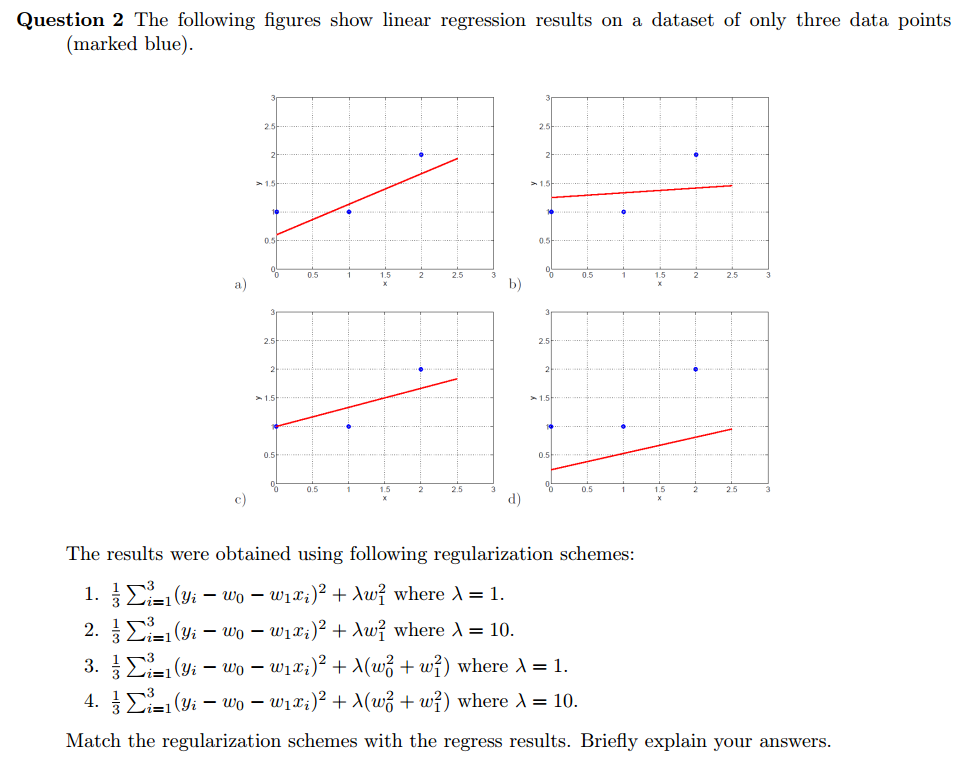
1. $\frac{1}{3} \sum_{i=1}^3 (y_i-\omega_0-\omega_1x_i)^2 + \lambda \omega_1^2$ where $\lambda=1$ —-> (c)
2. $\frac{1}{3} \sum_{i=1}^3 (y_i-\omega_0-\omega_1x_i)^2 + \lambda \omega_1^2$ where $\lambda=10$ —-> (b)
3. $\frac{1}{3} \sum_{i=1}^3 (y_i-\omega_0-w_1x_i)^2 + \lambda (\omega_0^2+\omega_1^2)$ where $\lambda=1$ —-> (a)
4. $\frac{1}{3} \sum_{i=1}^3 (y_i-\omega_0-\omega_1x_i)^2 + \lambda (\omega_0^2+\omega_1^2)$ where $\lambda=10$ —-> (d)

Explanation If we give the linear regression line an equation $y=kx+b$ then the $\omega_0$ is $b$ and the $\omega_1$ is $k$. The (c) line has lower slope because the $1\cdot \omega_1^2$ will make slope smaller. However too big $\lambda = 10$ will cause nearly no slope in the (b) line. If we add $w_0^2$ to the regularization, it causes both $b$ and $k$ decay. Compared to (1), the answer would be (a) line which has smaller $b$. Obviously, (4) will match (d) line because both $b$ and $k$ are small and the line is underfitting.

Question 3

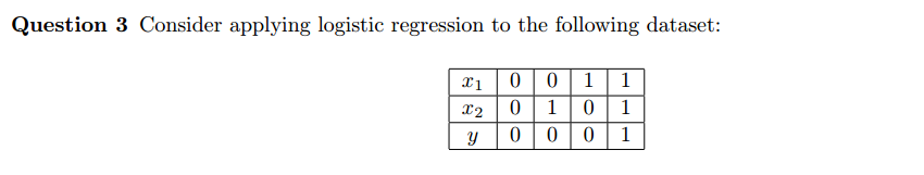
Like Question 1, writing down the matrix $X$ and $y$:

$$X = \begin{bmatrix} 1 & 0 & 0\\ 1 & 0 & 1\\ 1 & 1 & 0\\ 1 & 1 & 1 \end{bmatrix} \quad y = \begin{bmatrix} 0 \\ 0 \\ 0 \\ 1 \end{bmatrix}$$

Use batch gradient descent algorithm, get the parameter $\omega$ freshing formula

$$\omega_j=\omega_j+\alpha \sum_{i=1}^4[y_i-\sigma(\omega_0+\omega_1 x_1+\omega_2 x_2)]\cdot x_{i,j}$$

Suppose $\omega_0 = -2$, $\omega_1 = 1$ and $\omega_2 = 1$ initially and $\alpha = 0.1$. So we can calculate

$$\begin{aligned} \omega_0 = -2 + 0.1\cdot \{& [0-\sigma(-2+0+0)] \cdot 1 +\\ & [0-\sigma(-2+0+1)] \cdot 1 + \\ & [0-\sigma(-2+1+0)] \cdot 1 + \\ & [1-\sigma(-2+1+1)] \cdot 1 \} = -2.02 \end{aligned}$$

Similarly, we can calculated

$$\omega_1 =1.02 \quad \omega_2 = 1.02$$

Use sigmoid function

$$\begin{aligned} \hat{y_1} &= \sigma(\omega_0+\omega_1 \cdot 0+\omega_2 \cdot 0) = 0.12 \quad having \ 12\% \ chance \ in \ class \ 1 \ (belong \ to \ class \ 0)\\ \hat{y_2} &= \sigma(\omega_0+\omega_1 \cdot 0+\omega_2 \cdot 1) = 0.27 \quad having \ 27\% \ chance \ in \ class \ 1 \ (belong \ to \ class \ 0)\\ \hat{y_3} &= \sigma(\omega_0+\omega_1 \cdot 1+\omega_2 \cdot 0) = 0.27 \quad having \ 27\% \ chance \ in \ class \ 1 \ (belong \ to \ class \ 0)\\ \hat{y_4} &= \sigma(\omega_0+\omega_1 \cdot 1+\omega_2 \cdot 1) = 0.51 \quad having \ 51\% \ chance \ in \ class \ 1 \ (belong \ to \ class \ 1) \end{aligned}$$

The class distribution is [0, 0, 0, 1] so the training error = 0%

Question 4

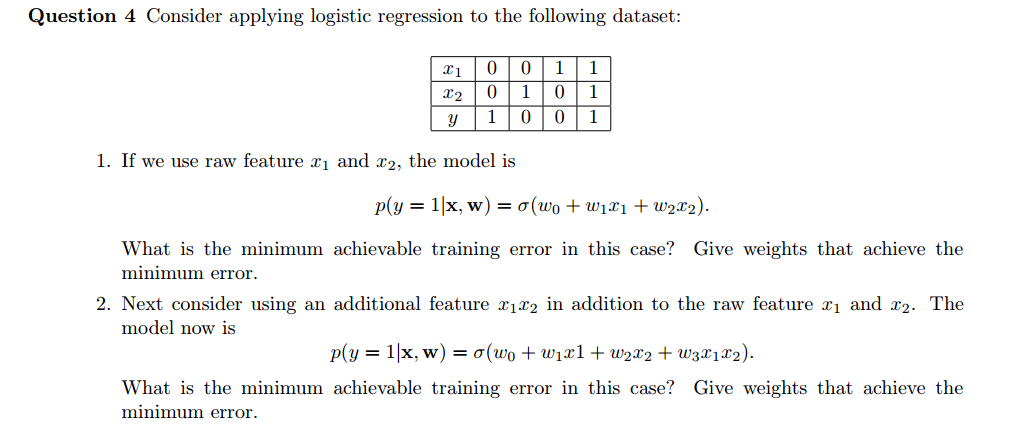
use raw features

If we use only raw features to classify, we would find that it’s a linear-inseparable question. This is because that we cannot find a surface to distinguish the positive and the negative. I use \textit{numpy} to help me calculate the batch gradient descent (BGD) process.

X4 = np.array([[1,0,0],
  [1,0,1],
  [1,1,0],
  [1,1,1]])
y4 = np.array([1,0,0,1])
w4 = np.array([-2,1,1])
a = 0.1
for i in range(100):
    w4 = w4 + 0.1 * (y4 - sc.expit(w4.dot(X4.T))).dot(X4)
    print(w4) # weight
    print(sc.expit(w4.dot(X4.T))) # y_predict

No matter how many iterations I run, the minimum error only achieves 1. After 100 iterations,

weight = [-0.3395675   0.28609699  0.28609699]
y_predict = [0.41591454 0.48663556 0.48663556 0.55789577]

After 1,000 iterations,

weight = [-2.23876505e-07  1.88743639e-07  1.88743639e-07]
y_predict = [0.49999994 0.49999999 0.49999999 0.50000004]

add an additional feature

However, if we add an additional feature, it’s equivalent to that projecting features from 2D to 3D. This makes the problem become linear-separable. Using the following code, after doing approximately 130 iterations, we can get a model having 0 trainning error (minimum training error).

X5 = np.array([[1,0,0, 0],
  [1,0,1, 0],
  [1,1,0, 0],
  [1,1,1, 1]])
y5 = np.array([1,0,0,1])
w5 = np.array([-2,1,1, 1])
a = 0.1
for i in range(130):
    w5 = w5 + 0.1 * (y5 - sc.expit(w5.dot(X5.T))).dot(X5)
    print(w5)
    print(sc.expit(w5.dot(X5.T)))

The weight and y_predict after 130 iterations,

weight = [ 0.0819811  -0.97091908 -0.97091908  3.39687673]
y_predict = [0.5204838  0.29132904 0.29132904 0.82303106]

Question 5

$$\omega_1 = \omega_1 + \alpha \sum_{i=1}^N[y_i-\sigma({\omega}^T {x}_i)]x_{i,1}$$

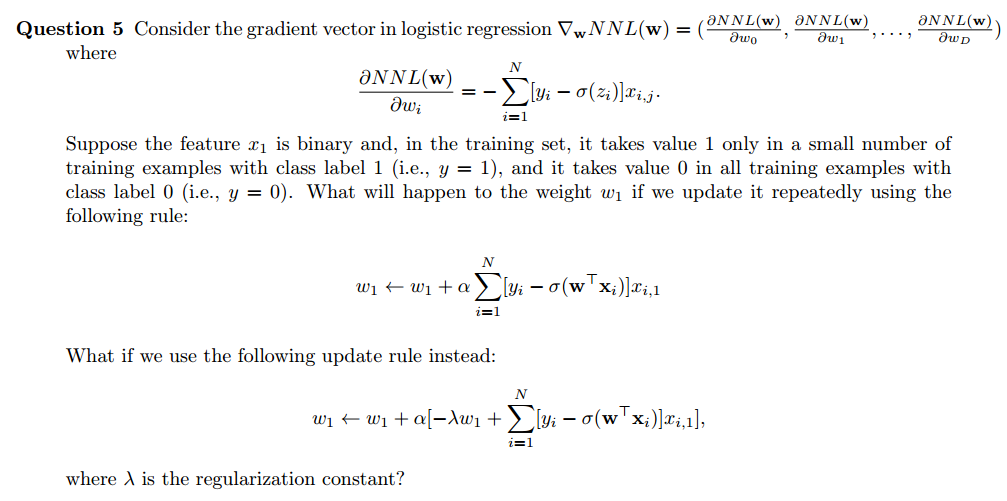
If predicted value $\sigma({\omega}^T {x}_i)$ is smaller than the actual value $y_i$, there is reason to increase $w_j$. The increment is proportional to $x_{i,1}$. If predicted value $\sigma({\omega}^T {x}_i)$ is larger than the actual value $y_i$, there is reason to decrease $w_j$. The decrement is proportional to $x_{i,1}$.

However, the question has already supposed the feature $x_1$ is binary whose value is unbalanced. The zero value of $x_1$ keeps the $w_1$ from \textit{learning} features from the example with LABEL 0. Otherwise, the $\omega_1$ would adjust according to both two classes. Therefore, this rule will force the model to fit example with a small number of training examples with LABEL 1 ( special feature in training set ). This causes \textbf{overfitting}.

$$\omega_1 = \omega_1 + \alpha \left[-\lambda \omega_1 + \sum_{i=1}^N[y_i-\sigma({\omega}^T{x}_i)]x_{i,1}\right]$$

Then adding the regularization constant is able to \textbf{reduce overfitting}. It helps the model not to learn too much from the training set. In the update rule, the $-\lambda \omega_1$ is independent, not influenced by the feature $x_1$.