Normalization is a big and important topic in machine learning so in this article I collect three important normalization methods which are batch norm, layer norm and group norm. I would also display how the normalizaiton work using CS231n codes as examples.
The following figure virtualizes the difference among batch norm, layer norm and group norm.
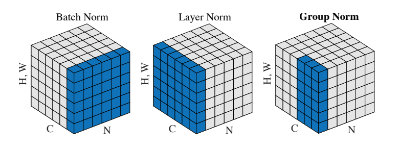
Normalization methods . N as the batch axix, C as the channel axis (Dimension), (H,W) as spatial axes - image height and width. The pixels in blue are normalized by the same mean and variance, computed by aggregating the values of these pixels.
1 The Comparison of BN, LN and GN
- BN - batch normalization
- LN - layer normalization
- GN - group normalization
Now we have
- $X$ : Matrix, mini-batch data of shape (N, D)
- $\gamma$ : Scale parameter
- $\beta$ : Shift paremeter
N is the number of samples in a batch, and D is the number of features. And $x_{i,j}$ to represent the element in matrix X.
2 Forward
Batch Normalization ( BN )
The python code1
2
3
4
5
6
7
8
9# x: Data of shape (N, D)
# gamma: Scale parameter of shape (D,)
# beta: Shift paremeter of shape (D,)
N, D = x.shape
mean = np.mean(x, axis=0, keepdims=True) # (1, D)
var = np.var(x, axis=0, keepdims=True) # (1, D)
x_norm = (x - mean) / np.sqrt(var + eps) # (N, D)
out = x_norm * gamma + beta
Layer Normalization ( LN )
Batch normalization has proved to be effective in making networks easier to train, but the dependency on batch size makes it less useful in complex networks which have a cap on the input batch size due to hardware limitations.
Several alternatives to batch normalization have been proposed to mitigate this problem; one such technique is Layer Normalization. Instead of normalizing over the batch, we normalize over the features. In other words, when using Layer Normalization, each feature vector corresponding to a single datapoint is normalized based on the sum of all terms within that feature vector.
Layer Normalization Ba, Jimmy Lei, Jamie Ryan Kiros, and Geoffrey E. Hinton. “Layer Normalization.” stat 1050 (2016): 21.
The LN’s formula is very similar to BN, just the across dimension is different.
The python code1
2
3
4
5N, D = x.shape
mean = np.mean(x, axis = 1, keepdims = True) # (N, 1)
var = np.var(x, axis = 1, keepdims = True) # (N, 1)
x_norm = (x - mean) / np.sqrt(var + eps) # (N, D)
out = x_norm * gamma + beta
Spatial Batch Normalization ( SBN )
The BN input data shape is (N, D). But for the CNN’s layer, it receives input data with shape (N, C ,H, W) and produce outputs of shape (N, C ,H, W) where the N dimension gives the minibatch size and the (H, W) dimensions give the spatial size of the feature map. Therefore, We need to tweak the BN a bit, then we will get SBN ( Spatial Batch Normalization ).
The python code, calling BN function. We need to transpose and reshape before sending the parameter into the batchnorm_forward() function.1
2
3
4N, C, H, W = x.shape
x_bn = x.transpose((0,2,3,1)).reshape(-1,C)
out_bn = batchnorm_forward(x_bn, gamma, beta, bn_param)
out = out_bn.reshape(N,H,W,C).transpose((0,3,1,2))
numpy.transpose is exchanging the sequence of axis. The original axis sequence is N, C, H, W. After using transpose((0,2,3,1)), the sequence becomes N, W, H, C. The we use reshape(-1, C) to make the matrix become 2 dimension —- the x_bn shape is ( N * W * H, C ).
Group Normalization ( GN )
In the previous part, we mentioned that Layer Normalization is an alternative normalization technique that mitigates the batch size limitations of Batch Normalization. However, as the authors of Ba, Jimmy Lei, Jamie Ryan Kiros, and Geoffrey E. Hinton. “Layer Normalization.” stat 1050 (2016): 21. observed, Layer Normalization does not perform as well as Batch Normalization when used with Convolutional Layers.
The authors of Wu, Yuxin, and Kaiming He. “Group Normalization.” arXiv preprint arXiv:1803.08494 (2018). propose an intermediary technique. In contrast to Layer Normalization, where you normalize over the entire feature per-datapoint, they suggest a consistent splitting of each per-datapoint feature into G groups, and a per-group per-datapoint normalization instead.
Even though an assumption of equal contribution is still being made within each group, the authors hypothesize that this is not as problematic, as innate grouping arises within features for visual recognition. One example they use to illustrate this is that many high-performance handcrafted features in traditional Computer Vision have terms that are explicitly grouped together. Take for example Histogram of Oriented Gradients N. Dalal and B. Triggs. Histograms of oriented gradients for human detection. In Computer Vision and Pattern Recognition (CVPR), 2005.— after computing histograms per spatially local block, each per-block histogram is normalized before being concatenated together to form the final feature vector.
The python code
1 | N, D = x.shape |
Spatial Group Normalization ( SGN )
We can understand the nature of SGN by comparing with BN / SBN.
The python code1
2
3
4
5
6
7N, C, H, W = x.shape
x_group = np.reshape(x, (N, G, C//G, H, W))
mean = np.mean(x_group, axis = (2, 3, 4), keepdims = True)
var = np.var(x_group, axis = (2, 3, 4), keepdims = True)
x_groupnorm = (x_group - mean) / np.sqrt(var + eps)
x_norm = np.reshape(x_groupnorm, (N, C, H, W))
out = x_norm * gamma + beta
C//G is that C is divided by G. axis=(2,3,4) is that do meaning to axis 2,3,4 one by one.